Forecasting with LSTM and explanatory time series

This tutorial example presents how to handle non-linear dependencies between a target and an explanatory time series using a LSTM neural network.

The calibration of the LSTM neural network relies on the raw traning set that is deemed to be trend-stationnary.

In this example, we use a simple sine-like signal onto which we added a synthetic linear trend.

Import libraries

Import the various libraries that will be employed in this example.

import copy
import pandas as pd
import numpy as np
import matplotlib.pyplot as plt
from pathlib import Path
from pytagi import Normalizer as normalizer
import pytagi.metric as metric

Import from Canari

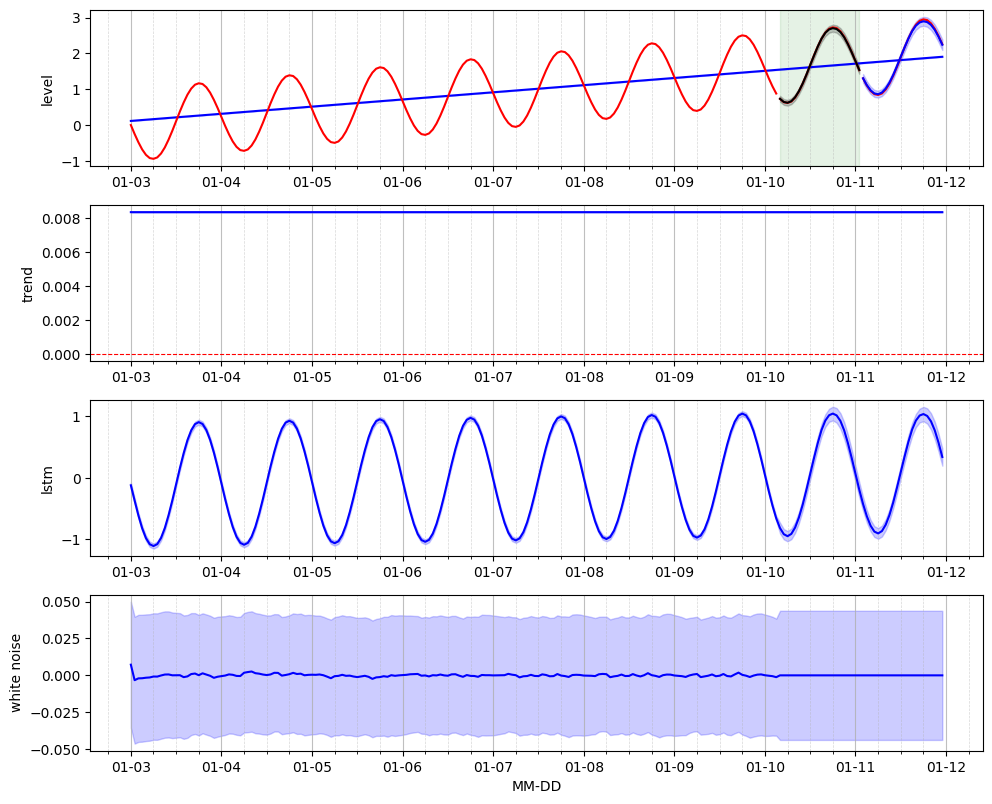
From Canari, we need to import several classes that will be reused in this example. Notably, we need to import the components that will be used to build the model; In terms of baseline, we use the LocalTrend and components. The recurrent pattern is modelled using a LstmNetwork and the residual is modelled by a WhiteNoise compoment.

from canari import (
    DataProcess,
    Model,
    plot_data,
    plot_prediction,
    plot_states,
)
from canari.component import LocalTrend, LstmNetwork, WhiteNoise

Read data

The raw .csv data is saved in a dataframe using the Panda external library.

project_root = Path.cwd().resolve().parents[1]
data_file = str(project_root / "data/toy_time_series/sine.csv")
df = pd.read_csv(data_file, skiprows=1, delimiter=",", header=None)
# Add a trend to the data
linear_space = np.linspace(0, 2, num=len(df))
df = df.add(linear_space, axis=0)
#
data_file_time = str(project_root / "data/toy_time_series/sine_datetime.csv")
time_index = pd.read_csv(data_file_time, skiprows=1, delimiter=",", header=None)
time_index = pd.to_datetime(time_index[0])
df.index = time_index
df.index.name = "time"
df.columns = ["values"]
df.head()

	values
time
2000-01-03 00:00:00	0.000000
2000-01-03 01:00:00	-0.250698
2000-01-03 02:00:00	-0.481395
2000-01-03 03:00:00	-0.682093
2000-01-03 04:00:00	-0.832791

Add dependent variables

We define the dependent explanatory variables as the moving average with window-lenght equal to 3 and a lag of two time steps.

# Add columns with lagged values
lag = [2]
df = DataProcess.add_lagged_columns(df, lag)

# Add moving average
df['Moving_Average'] =  df['values'].rolling(window=3).mean()
df.head()

	values	values_lag1	values_lag2	Moving_Average
time
2000-01-03 00:00:00	0.000000	0.000000	0.000000	NaN
2000-01-03 01:00:00	-0.250698	0.000000	0.000000	NaN
2000-01-03 02:00:00	-0.481395	-0.250698	0.000000	-0.244031
2000-01-03 03:00:00	-0.682093	-0.481395	-0.250698	-0.471395
2000-01-03 04:00:00	-0.832791	-0.682093	-0.481395	-0.665426

Data preprocess

In terms of pre-processsing, we define here our choice of using the first 80% of the raw time series for trainig and the following 10% for the validaiton set. The remaining last 10% are the implicitely defined as the test set.

output_col = [0]
data_processor = DataProcess(
    data=df,
    train_split=0.8,
    validation_split=0.1,
    output_col=output_col,
)
train_data, validation_data, test_data, standardized_data = data_processor.get_splits()

Define model from components

We instantiatiate each component brom their base class. The local_trend baseline component relies on the default hyperparameters. The recurrent pattern will use a 1-layer LSTM neural network with 50 hidden units with a look-back length of 19 time steps. The look-back window consists in the set of past neural network’s outputs that are employed as explanatory variables in order to predict the current output. In addition there are 4 features that are used as explanatory variables. The residual is modelled by a Gaussian white noise with a mean 0 and a user-defined standard deviation of 0.05.

Note that we use auto_initialize_baseline_states in order to automatically initialize the baseline hidden states based on the first day of data.

local_trend = LocalTrend()
pattern = LstmNetwork(
        look_back_len=19,
        num_features=4,  # number of data's columns + time covariates
        num_layer=1,
        num_hidden_unit=50,
        device="cpu",
        manual_seed=1,
    )
residual = WhiteNoise(std_error=0.05)

model = Model(local_trend, pattern, residual)
model.auto_initialize_baseline_states(train_data["y"][0 : 24])

Training the LSTM neural network

The training of the LSTM neural network model is done using the training and validation sets. The training set is used to perform the time series decomposition into a baseline, pattern and residual and to simultanously learn the LSTM neural network parameters. The validation set is used in order to identify the optimal training epoch for the LSTM neural network. Note that it is essential to perform this training on a dataset that is either stationnary or trend-stationnary.

num_epoch = 50
for epoch in range(num_epoch):
    (mu_validation_preds, std_validation_preds, states) = model.lstm_train(
        train_data=train_data,
        validation_data=validation_data,
    )

    # Unstandardize the predictions
    mu_validation_preds = normalizer.unstandardize(
        mu_validation_preds,
        data_processor.scale_const_mean[output_col],
        data_processor.scale_const_std[output_col],
    )
    std_validation_preds = normalizer.unstandardize_std(
        std_validation_preds,
        data_processor.scale_const_std[output_col],
    )

    # Calculate the log-likelihood metric
    validation_obs = data_processor.get_data("validation").flatten()
    mse = metric.mse(mu_validation_preds, validation_obs)

    # Early-stopping
    model.early_stopping(evaluate_metric=mse, current_epoch=epoch, max_epoch=num_epoch)
    if epoch == model.optimal_epoch:
        mu_validation_preds_optim = mu_validation_preds
        std_validation_preds_optim = std_validation_preds
        states_optim = copy.copy(
            states
        )
        lstm_optim_states = model.lstm_net.get_lstm_states()

    model.set_memory(states=states, time_step=0)
    if model.stop_training:
        break

Set relevant variables for predicting in the test set

In order to forecast on the test set, we need to set the LSTM and SSM states to the values corresponding to the last time step of the validation set. Note that the values corresponds to those associated with the optimal training epoch as identified using the validation set.

model.lstm_net.set_lstm_states(lstm_optim_states)
model.states = states_optim
model.set_memory(
    states=states_optim,
    time_step=data_processor.test_start,
)

Forecast on the test set

We perform recursive 1-step ahead forecasts on the test set and then proceed with un-standardization of the data in order to retreive the original scale of the raw data.

mu_test_preds, std_test_preds, states = model.forecast(
    data=test_data,
)

# Unstandardize the predictions
mu_test_preds = normalizer.unstandardize(
    mu_test_preds,
    data_processor.scale_const_mean[output_col],
    data_processor.scale_const_std[output_col],
)
std_test_preds = normalizer.unstandardize_std(
    std_test_preds,
    data_processor.scale_const_std[output_col],
)

Predictions and hidden states

We represent the time-series decomposition visually where the raw data is overlaid with the baseline hidden state represented by the level. The rate of change of the baseline is characterized by the trend hidden states. The recurrent pattern is captured by the LSTM neural network. The posterior estimate for the residuals are displayed for the white noise component. The forecast period corresponds to the last day of data following the validation set, which is depicted by the green-shaded region.

fig, ax = plot_states(
    data_processor=data_processor,
    states=states,
    )
plot_data(
    data_processor=data_processor,
    plot_train_data=True,
    plot_test_data=True,
    plot_validation_data=True,
    sub_plot=ax[0]
    )
plot_prediction(
    data_processor=data_processor,
    mean_validation_pred=mu_validation_preds,
    std_validation_pred = std_validation_preds,
    sub_plot=ax[0],
    color="k",
    )
plot_prediction(
    data_processor=data_processor,
    mean_test_pred=mu_test_preds,
    std_test_pred = std_test_preds,
    sub_plot=ax[0],
    color="b",
    )
ax[-1].set_xlabel("MM-DD")
plt.show()