Univariate time series forecasting without LSTM

This tutorial example presents how to perform forecasts for an univariate time series while using a simple fourrier-form periodic component rather than a LSTM neural network.

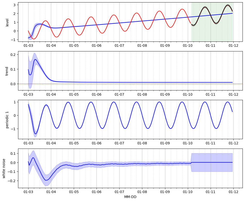
In this example, we use a simple sine-like signal onto which we added a synthetic linear trend.

Import libraries

Import the various libraries that will be employed in this example.

import pandas as pd
import numpy as np
import matplotlib.pyplot as plt
from pathlib import Path

Import from Canari

From Canari, we need to import several classes that will be reused in this example. Notably, we need to import the components that will be used to build the model; In terms of baseline, we use the LocalTrend and components. The recurrent pattern is modelled using a Periodic component, and the residual is modelled by a WhiteNoise compoment.

from canari import (
    DataProcess,
    Model,
    plot_data,
    plot_prediction,
    plot_states,
)
from canari.component import LocalTrend, Periodic, WhiteNoise

Read data

The raw .csv data is saved in a dataframe using the Panda external library.

project_root = Path.cwd().resolve().parents[1]
data_file = str(project_root / "data/toy_time_series/sine.csv")
df = pd.read_csv(data_file, skiprows=1, delimiter=",", header=None)
# Add a trend to the data
linear_space = np.linspace(0, 2, num=len(df))
df = df.add(linear_space, axis=0)
#
data_file_time = str(project_root / "data/toy_time_series/sine_datetime.csv")
time_index = pd.read_csv(data_file_time, skiprows=1, delimiter=",", header=None)
time_index = pd.to_datetime(time_index[0])
df.index = time_index
df.index.name = "time"
df.columns = ["values"]

Data preprocess

In terms of pre-processsing, we define here our choice of using the first 80% of the raw time series for trainig and the following 20% for the validaiton set.

output_col = [0]
data_processor = DataProcess(
    data=df,
    train_split=0.8,
    validation_split=0.2,
    output_col=output_col,
    standardization=False,
)
train_data, validation_data, test_data, standardized_data = data_processor.get_splits()
data_processor.data.head()

	values
time
2000-01-03 00:00:00	0.000000
2000-01-03 01:00:00	-0.250698
2000-01-03 02:00:00	-0.481395
2000-01-03 03:00:00	-0.682093
2000-01-03 04:00:00	-0.832791

Define model from components

We instantiatiate each component brom the corresponding class. The local_trend baseline component relies on the default hyperparameters. The recurrent pattern will use Fourrier-form Periodic component. The residual is modelled by a Gaussian white noise with a mean 0 and a user-defined standard deviation of 0.1.

Note that we use auto_initialize_baseline_states in order to automatically initialize the baseline hidden states based on the first day of data.

local_trend = LocalTrend()
pattern = Periodic(mu_states=[0,0],var_states=[1,1],period=24)
residual = WhiteNoise(std_error=0.1)

model = Model(local_trend, pattern, residual)
model.auto_initialize_baseline_states(train_data["y"][0 : 24])

Filter on train data

We perform recursive SSM 1-step ahead prediction- and update-steps using the Kalman filter over the entire training set.

mu_train_pred, std_train_pred, states=model.filter(data=train_data)

Forecast on validation data

We perform recursive 1-step ahead forecasts on the validatiobn set.

mu_val_pred, std_val_pred, states=model.forecast(data=validation_data)

Predictions and hidden states

We represent the time-series decomposition visually where the raw data is overlaid with the baseline hidden state represented by the level. The rate of change of the baseline is characterized by the trend hidden states. The recurrent pattern is captured by the LSTM neural network. The posterior estimate for the residuals are displayed by the white noise component. The forecast period corresponds to the last two days within the validation set is depicted by the green-shaded region.

fig, ax = plot_states(
    data_processor=data_processor,
    states=states,
    states_to_plot=["level","trend","periodic 1", "white noise"]
    )
plot_data(
    data_processor=data_processor,
    plot_train_data=True,
    plot_test_data=False,
    plot_validation_data=True,
    sub_plot=ax[0]
    )
plot_prediction(
    data_processor=data_processor,
    mean_validation_pred=mu_val_pred,
    std_validation_pred = std_val_pred,
    sub_plot=ax[0],
    color="k",
    )
ax[-1].set_xlabel("MM-DD")
plt.show()